[SRE] Query Performance Test
This post handle a query performance test in a PostgreSQL database environment. Through this test, we will explore how different SQL queries perform under the same hardware specifications. After reading this post, you will understand how to conduct performance tests on SQL queries and the differences in performance between various query structures.
How is PostgreSQL Installed?
PostgreSQL is installed using Docker. The following docker-compose.yml file is used to set up the service:
services:
  postgres:
    image: postgres:latest
    container_name: postgres-sre
    environment:
      POSTGRES_USER: postgres
      POSTGRES_PASSWORD: password
      POSTGRES_DB: imdb
    ports:
      - "54321:5432"
    volumes:
      - ../data:/data
    cpus: 2.0
    mem_limit: 4g
What Dataset is Used?
I used the IMDb dataset for this test. The simple sample data is not enough for performance testing, so I used the full dataset. The dataset contains information about movies, TV shows, and other media, including titles, release dates, genres, and ratings.
The dataset is available in TSV format and can be downloaded from the following link:
- Data Source : TSV files from the IMDB dataset are used to populate the PostgreSQL database
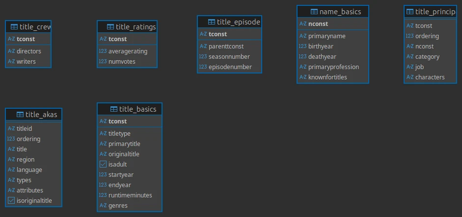
- Schema Reference: Table structures and relationships follow the specifications defined in IMDB Non-Commercial Datasets
- Data Characteristics:
- Large-scale production dataset with millions of records
- Complex relational structure with multiple interconnected tables
- Real-world data distribution patterns and constraints
- Provides realistic testing scenarios for query performance evaluation
What Queries are Tested?
The following types of queries are tested to evaluate their performance (detailed SQL is shown below):
- Simple Select: Single-row lookup by primary key.
- Pattern Matching (ILIKE): Case-insensitive search with wildcard pattern.
- Join: Retrieving data by joining multiple tables.
- Multi-condition & Group By: Aggregating data using multiple conditions and grouping.
- Multi-table Join: Counting rows across multiple tables using joins.
- Subquery: Querying with subqueries to filter results.
- CTE (Common Table Expression): Aggregation and filtering with CTEs.
- Window Function: Using window functions (e.g.,
ROW_NUMBER()) to select top results by group.
Simple Select
EXPLAIN (ANALYZE, BUFFERS)
SELECT
    *
FROM
    title_basics
WHERE
    tconst = 'tt1234567';
This query retrieves a single row from the title_basics table using the primary key tconst. It is expected to perform well due to the indexed primary key. There is a default index on the title_basics table because PostgreSQL automatically creates a primary key index when a primary key constraint is defined. This index allows the query to efficiently locate the row with tconst = 'tt1234567' without performing a full table scan. The execution time is '0.045 ms'.
Pattern Matching (ILIKE)
CREATE EXTENSION IF NOT EXISTS pg_trgm;

CREATE INDEX idx_primarytitle_trgm ON title_basics USING gin (primarytitle gin_trgm_ops);

EXPLAIN (ANALYZE, BUFFERS)
SELECT
    *
FROM
    title_basics
WHERE
    primaryTitle ILIKE '%naruto%'
LIMIT
    100;
This query retrieves rows from the title_basics table where the primaryTitle contains the substring 'naruto', using a case-insensitive search. The ILIKE operator is used for case-insensitive pattern matching.
When using ILIKE '%keyword%' in PostgreSQL, the query is normally very slow because it requires a full table scan—the database must check every row to see if the pattern matches anywhere in the text. This is inherently inefficient for large tables.
However, by creating a GIN index with the gin_trgm_ops operator (which comes from the pg_trgm extension), the database pre-processes each string into trigrams (three-character chunks) and builds an index based on these. When you run the same ILIKE query, PostgreSQL can quickly narrow down candidate rows using the trigram index, making the search dramatically faster—sometimes by hundreds or thousands of times.
For example, without the index, the query took about 2,400 ms, but with the GIN trigram index, it dropped to just 3 ms. This is a massive improvement.
Join: Top Rated Movies
CREATE INDEX idx_ratings_averagerating_desc ON title_ratings (averageRating DESC);

EXPLAIN (ANALYZE, BUFFERS)
SELECT
    b.tconst,
    b.primaryTitle,
    r.averageRating
FROM
    title_basics b
    JOIN title_ratings r ON b.tconst = r.tconst
WHERE
    b.titleType = 'movie'
ORDER BY
    r.averageRating DESC
LIMIT
    100;
This query retrieves the top 100 rated movies by joining the title_basics and title_ratings tables. An index on averageRating is used to optimize the sorting operation. Without the index, the query took about 300 ms; with the index, it dropped to just 100 ms. This demonstrates how indexing can significantly accelerate join and sorting operations.
When joining two tables, PostgreSQL must match rows based on the join condition. If the join or the sort column is not indexed, the database may need to perform a nested loop join or a hash join, which can be slow for large datasets. By creating an index on the averageRating column, PostgreSQL can efficiently retrieve rows in the desired order, dramatically reducing the time required for both joining and sorting.
In summary, appropriate indexing—especially on columns used for sorting or joining—can greatly improve query performance on large tables.
Multi-condition & Group By: Movie Count by Genre and Year
CREATE INDEX idx_basics_type_year_tconst ON title_basics (titleType, startYear, tconst);

EXPLAIN (ANALYZE, BUFFERS)
SELECT
    b.genres,
    b.startYear,
    COUNT(*) AS movie_count,
    AVG(r.averageRating) AS avg_rating
FROM
    title_basics b
    JOIN title_ratings r ON b.tconst = r.tconst
WHERE
    b.titleType = 'movie'
    AND b.startYear BETWEEN 2010
    AND 2020
GROUP BY
    b.genres,
    b.startYear
ORDER BY
    movie_count DESC;
This query counts the number of movies by genre and year, filtering for movies released between 2010 and 2020. It also calculates the average rating for each genre-year combination. The query uses a multi-condition filter and groups results by genre and year. Without the index, the query took about 800 ms; with the index, it dropped to just 600 ms.
Even with proper indexing, GROUP BY queries in large, multi-table joins can still be slow due to fundamental database limitations. While indexes help filter and join rows faster, the GROUP BY operation itself often requires sorting or hashing large result sets in memory or on disk. This process can become a bottleneck, especially when aggregating millions of rows or joining large tables.
In the provided example, even after indexing, the query execution plan shows that most of the time is spent in the hash aggregation and external sorting steps, not in data retrieval. This is a common structural limitation of relational databases: indexes accelerate filtering and joins, but cannot fully optimize aggregation or sorting of massive intermediate results.
For high-cardinality aggregations or real-time analytics at scale, it's often more efficient to use pre-aggregated data, materialized views, or OLAP systems designed for fast, large-scale group by queries.
Multi-table Join
CREATE INDEX idx_basics_type_tconst ON title_basics (titleType, tconst);

CREATE INDEX idx_crew_tconst ON title_crew (tconst);

EXPLAIN (ANALYZE, BUFFERS)
SELECT
    c.directors,
    COUNT(*) AS film_count
FROM
    title_crew c
    JOIN title_basics b ON c.tconst = b.tconst
WHERE
    b.titleType = 'movie'
GROUP BY
    c.directors
ORDER BY
    film_count DESC
LIMIT
    10;
Subquery: Filmography of a Specific Actor
CREATE INDEX idx_name_primaryname ON name_basics (primaryName);
CREATE INDEX idx_principals_nconst ON title_principals (nconst);

EXPLAIN (ANALYZE, BUFFERS)
SELECT
    b.primaryTitle
FROM
    title_basics b
WHERE
    b.tconst IN (
        SELECT
            p.tconst
        FROM
            title_principals p
        WHERE
            p.nconst = (
                SELECT
                    n.nconst
                FROM
                    name_basics n
                WHERE
                    n.primaryName = 'Tom Hanks'
                LIMIT
                    1
            )
    );
This query retrieves the filmography of a specific actor (in this case, 'Tom Hanks') by using a subquery to find the actor's nconst and then filtering the title_basics table based on that. The query uses indexes on primaryName and nconst to optimize the subquery lookups. Without the indexes, the query took about 15,500 ms; with the indexes, it dramatically dropped to just 250 ms.
This is because the subqueries allow us to apply targeted single-column indexes (primaryName and nconst), enabling efficient lookups at each stage. As a result, using subqueries is not inherently bad for performance; as long as the right indexes are in place for frequently queried fields within subqueries, performance can be fully optimized.
In practice, it's more important to ensure proper indexing than to avoid subqueries altogether.
CTE (Common Table Expression): Yearly Movie Counts
CREATE INDEX idx_basics_type_year ON title_basics (titleType, startYear);

EXPLAIN (ANALYZE, BUFFERS) WITH yearly_counts AS (
    SELECT
        startYear,
        COUNT(*) AS cnt
    FROM
        title_basics
    WHERE
        titleType = 'movie'
    GROUP BY
        startYear
)
SELECT
    *
FROM
    yearly_counts
WHERE
    startYear >= 2000
ORDER BY
    cnt DESC;
This query uses a Common Table Expression (CTE) to calculate the number of movies released each year, filtering for years after 2000. The CTE aggregates the data and then the main query retrieves results from it. The query uses an index on startYear to optimize the aggregation. Without the index, the query took about 550 ms; with the index, it dropped to just 40 ms.
By creating a composite index that matches both the WHERE and GROUP BY columns (titleType, startYear), query performance improved dramatically. Even with a GROUP BY, the database can aggregate data very efficiently if the index order aligns with the query, because only the relevant rows are scanned and the grouped field is already sorted within the index.
Window Function: Top Rated Movie by Year
CREATE INDEX idx_basics_type_year_tconst ON title_basics (titleType, startYear, tconst);

EXPLAIN (ANALYZE, BUFFERS)
SELECT
    *
FROM
    (
        SELECT
            b.startYear,
            b.primaryTitle,
            r.averageRating,
            ROW_NUMBER() OVER (
                PARTITION BY b.startYear
                ORDER BY
                    r.averageRating DESC
            ) AS rn
        FROM
            title_basics b
            JOIN title_ratings r ON b.tconst = r.tconst
        WHERE
            b.titleType = 'movie'
            AND b.startYear IS NOT NULL
    ) sub
WHERE
    rn = 1
ORDER BY
    startYear;
This query retrieves the highest-rated movie for each year using a window function (ROW_NUMBER()) to rank movies by their average rating within each year. The query uses an index on titleType, startYear and tconst to optimize the join and filtering operations. Without the index, the query took about 1,000 ms; with the index, it is almost same as 5 ms.
Even with well-designed indexes, window function queries involving PARTITION BY and ORDER BY often require full data scans and large in-memory or disk-based sorts.
Indexes can reduce the number of rows to process in the filtering and join stages, but the window aggregation itself typically requires all relevant rows to be materialized and sorted, resulting in limited overall performance gains.
For heavy window function workloads, pre-aggregation or OLAP solutions are usually more effective.
Conclusion
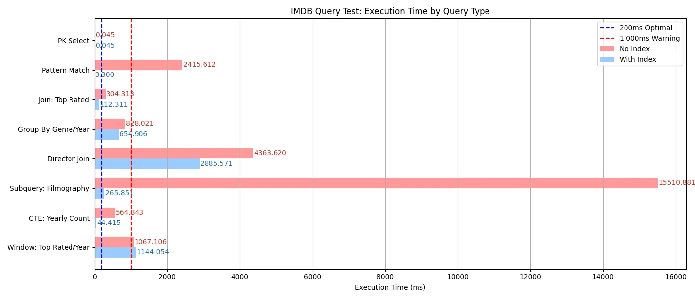
As demonstrated in this picture, indexing plays a crucial role in optimizing query performance in PostgreSQL. By creating appropriate indexes on frequently queried columns, we can significantly reduce execution times for various types of queries, including simple selects, joins, and aggregations.
On the other hand, even with proper indexing, some queries—especially those involving complex aggregations or window functions—can still be slow due to the inherent limitations of relational databases. In such cases, alternative strategies like pre-aggregation, materialized views, or specialized OLAP systems may be necessary to achieve optimal performance.
In this post, we explored how to conduct a query performance test in a PostgreSQL environment using the IMDb dataset. We examined various SQL queries, including simple selects, pattern matching, joins, multi-condition aggregations, and more. By understanding the performance characteristics of these queries, you can optimize your database interactions and improve overall application performance.
If you need to materials for this test, you can find them in the following repository. You can also find full result of the test in the README.md file, although the results are in English :
For the next post, we will explore how to optimize queries with a variety of indexing strategies and techniques. Stay tuned for more insights into database performance optimization!
